On Physical Significance of Spaces with Neutral Signature

Negative Energies in Classical Theories

We have seen that the Clifford space, C, is a manifold, whose tangent space at any of its points is the Clifford algebra $Cl(1,3)$ . Its metric has the signature (8,8), which means that it can be represented as the diagonal matrix with eight times $+1$ and eight times $-1$ . Minkowski space has signature (1,3) and is an example of a hyperbolic space. In general, spaces with a signature, $(p,q)$ , $p>1$ , are called ultra hyperbolic spaces. If $p=q$ , the space is called to have neutral signature. The Clifford space C is an example of a space with neutral signature. Ultra hyperbolic spaces are generally believed to be unsuitable for physics, because they imply negative energies. I will demonstrate that negative energies, if properly treated, can make sense in physics. One known example is the Dirac theory of a relativistic particle, where the issue of negative energies was successfully resolved, although initially it presented a rather big puzzle [1]. Here I will talk about other cases, where negative energies are still considered as problematic. I will discuss a simple system in two dimensions. Generalization to higher dimensions and field theory is straightforward.

Harmonic oscillator in the space $M_{1,1}$

1. Free oscillator, without interaction
Let us consider the harmonic oscillator described by the Lagrangian

(1) $L =\frac{1}{2}\, (\dot x^2 -\dot y^2) -\frac{1}{2}\, \omega^2 (x^2 - y^2)$ .

The corresponding equations of motion are

(2) $\ddot x + \omega x = 0,~~~~\ddot y + \omega y=0$

We see that the change of sign in front of the y-term in the Lagrangian has no influence on the equations of motion.

The canonical momenta are

(3) $p_x = \frac{{\partial L}}{{\partial\dot x}} = \dot x\,~~~~p_y = \frac{{\partial L}}{{\partial \dot y}} = -\dot y$

and the Hamiltonian is

(4) $H = p_x \dot x + p_y \dot y - L = \frac{1}{2}(p_x^2 - p_y^2) + \frac{{\omega^2}}{2}(x^2 - y^2)$ .

It can be positive or negative, but this does not mean that the system is unstable. Namely, the Hamilton equation of motion are now

(5) ${\ddot x} = - \frac{\partial V}{\partial x}~,~~~~~~~ {\ddot y} = \frac{\partial V}{\partial y}~,~~~~ V=\frac{{\omega^2}}{2}(x^2 - y^2)$ .

Notice that the y-equation has different sign in front of the force term than has the x-equation. This is the reason that also the motion of the y-component is stable, because it is described by the equation of motion of the form (2). The criterion for stability of the $y$ -degree of freedom is that the potential must have a maximum in the $(y,V)$ -plane [2-4]. We see that the usual intuition, namely that the system is stable if the potential has minimum, does not hold for the degrees of freedom with negative energy. For such degrees of freedom, the system is stable if the potential has maximum.

Among certain experts [4-7] it is well known that the system, described by the Lagrangian (1), and other analogous, more general systems in field theory, are not problematic neither in the classical nor in the quantized theory, provided that there is no interaction between the degrees of freedom with positive and negative energy. But if one switches on an interaction, then, according to the wide spread belief, the system unavoidably becomes unstable so that its position and velocity escape into infinity. We shall now demonstrate that this is not always the case, and that even in the presence of interactions, the system with positive and negative energy degrees of freedom can be stable.

2. Presence of interactions

In general, the interacting oscillator in the space $M_{1,1}$ is given by

(6) $L = \frac{1}{2}(\dot x^2 - \dot y^2) - V$
(7) $V = \frac{\omega}{2}(x^2 - y^2) + V_1$ .

Let us now consider the case of the interaction

(8) $V_1 = \frac{\lambda }{4}(x^2 - y^2)^2$ .

The equations of motion are then

(9) $\ddot x + \omega ^2 x + \lambda \,x (x^2 - y^2) =0$ ,
(10) $\ddot y + \omega ^2 y + \lambda \,y (x^2 - y^2 ) = 0$ .

These equations can be solved numerically by the program Mathematica. Let us take $\omega =1$ and $\lambda = 0.1$ , and the initial conditions ${\dot x} (0)=1$ , ${\dot y}(0)=0$ , $x(0)=0$ , $y(0)=1$ . In the figure below it is shown how the trajectory in the $(x,y)$ space starts to evolve in time. The time period in this figure is from $t=0$ to $t=25$ . The units are arbitrary.

If we take a longer time period, e.g., from $t=0$ to $t=100$ , then we obtain the following picture:

We see that at $t=100$ , the amplitudes of oscillations are $x\approx 10$ and $y\approx 10$ , whereas at t=25 the amplitudes were x=1.2 and y=1.2. Numerical calculations for larger values of t reveal that the system is unstable in the sense that the amplitudes of $x(t), y(t)$ , ${\dot x}(t)$ , $\dot y(t)$ grow to infinity. In the figure bellow it is shown how the kinetic energy ${\dot x}^2/2$ increases with time.

Such results, of course, were expected, because the system described by the Lagrangian (6)-(8) has negative energies, and it is well known that negative energies imply instability. However, the total energy,

(11) $E_{\rm tot}=\frac{1}{2}({\dot x}^2 - {\dot y}^2)+V(x,y)$ ,

remains constant. For the above numerical solution, this is confirmed in the following figure, where the total energy remains constant within numerical error.

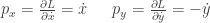
If we change the initial conditions or the coupling constant $\lambda$ , then we obtain, of course, different solutions that also escape into infinity. An interesting alternative to the $(x,y)$ diagram above, that I do not show here, can be found in Ref. [8].

Let us now consider slightly modified equations of motion by introducing two constants $\mu$ and $\nu$ :

(12) $\ddot x + \mu [\omega^2 x + \lambda \,x (x^2 - y^2)] = 0$ ,

(13) $\ddot y + \nu [\omega^2 y + \lambda \,y (x^2 - y^2)] = 0$ .

The solution for 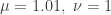$\mu = 1.01,~\nu = 1$ , and the same initial conditions as before, is [8]:

Left: trajectories in the $(x,y)$ . space. Right: the kinetic energy ${\dot x}^2/2$ as function of time.

Now something really fascinating has happened: The system is no longer unstable! We see that the trajectory in the $(x, y)$ space does not escape into infinity. Instead, a second arm is formed, and the trajectory remains confined within a star-like envelope. The kinetic energy of one component, ${\dot x}^2/2$ , now does not grow to infinity. Instead, the amplitude of the kinetic energy oscillations is modulated by a slowly oscillating envelope. Rapid oscillations within the envelop are not visible in the diagram.

In the lower part of the latter figure we repeat the calculation for $\mu=1.0001$ and $\nu =1$ . This is now very close to $\mu=1$ , $\nu=1$ , the case of Eqs. (9),(10). Now the trajectory in the $(x,y)$ space goes much farther from the origin than in the case $\mu=1.01$ . But again it does not go to infinity; instead, after some time, the trajectory start to move within a second arm. The envelope of the kinetic energy oscillations now consists of separated peaks. As $\mu$ approaches $1$ , the height of the peaks becomes higher and higher, and their separation increases. In the limit $\mu \to 1$ , the height of the first peak is infinite, and there is no second or other peaks (because their positions recedes to infinity). This is a singular case, in which the system is unstable. But if $\mu$ slightly differs from $\nu$ , then the system is stable; its trajectory remains confined within a finite region of the $(x,y)$ space, and the kinetic energy remains finite as well.

3. Collision of the oscillator with a free particle

Let us assume that in the surroundings of the oscillator, O, described by the Lagrangian (6)-(8), there is free particle, P. Depending on the initial conditions, it may happen that the oscillator hits the particle. Such a combined system of O and P can be modeled by the Lagrangian given in the next figure.

Click on figure to enlarge it

*See footnote

Let us solve this system for the constants $\lambda =0.1~$ , $\alpha=1$ , and the initial conditions $\dot x(0) = 1$ , $~~\dot y(0) = 0$ , $~~\dot u(0) = 0$ , $~~\dot v(0) = 0$ , $x(0) = 0$ , $~~y(0) = 1$ , $~~u(0) = 12$ , $~~v(0) = 11.5$ . The results are shown in this picture:

We see that the solution properly reproduces the fact that the particle $P$ is initially at rest, and after the interaction with the oscillator $O$ , it moves with a constant velocity. The total energy of the system remains constant, as shown in the lower left diagram of the above figure.

The positive component of the oscillator’s kinetic energy starts to increase, but at time around $t=112$ it drops down to zero, because the energy was transferred to the particle $P$ . After a while, the oscillator “recovers”, and its positive energy starts to increase again. A further collision with some other particle would again drop down ${\dot x}^2/2$ . Analogous holds for ${\dot y}^2/2$ . We see that, according to this numerical solution, the surrounding particles stabilize the oscillator and prevent it to escape into the infinity. We expect that many such oscillators, immersed into a bath of particles would increase their average ${\dot u}^2/2$ and ${\dot v}^2/2$ , i.e., the temperature of the bath. We see that this is a fascinating system, and it would be even more fascinating, if such systems could actually exist in nature (see a discussion at the end of Ref. [8]).

In the following posts I intend to say more on the fascinating world of negative energies. Among others, I will point out that negative energies also occur in the systems described by higher derivatives, and that such systems are not so problematic as it has been believed so far [9],[10].

[1] E. Fermi 1932 Rev. Mod. Phys. 4 87.
[2] M. Pavšič 1999 Phys. Lett. A 254 119 [hep-th/9812123].
[3] M. Pavšič 2005 Found. Phys. 35 1617 [hep-th/0501222].
[4] R. Woodard 2007 Lect. Notes Phys. 720 403.
[5] W. Pauli 1943 Rev. Mod. Phys. 15 175.
[6] D. Cangemi, R. Jackiw, and B Zwiebach 1996 Annals of Physics 245 408.
[7] E. Benedict, R. Jackiw and H.J. Lee 1996 Phys. Rev. D 54 6213
[8] M. Pavšič J. Phys. Conf. Ser. 437 012006 (2013) arXiv:1210.6820 [hep-th].
[9] M. Pavšič 2013 Mod. Phys. Lett. A 28 1350165 arXiv:1302.5257 [gr-qc]
[10] M. Pavšič 2013 Phys. Rev. D 87 107502 arXiv:1304.1325 [gr-qc].

*In this figure we corrected the sign in front of the last term in the y-equation. The correct sign is minus, whereas in the initial version of this post the sign was plus. The wrong sign is also in Ref.[8], Eq. (89). This is a typo. The calculation was done with the correct minus sign in the y-equation.

2 Responses to On Physical Significance of Spaces with Neutral Signature

amarashiki says:

October 28, 2013 at 21:34

From a pure physical viewpoint, how do you avoid the quantum instability you get due to negative energies, i.e., to the instability associated to have energies not bounded from below? It seems “problematic” at least from the common notion of (quantum) stability…

- Matej Pavšič says:
  
  October 29, 2013 at 13:22
  
  See explanation after Eq. (5) of this post. In the case of negative energies, the system is stable if the potential is bounded from above, not from below. This also holds in the quantum theory. For a free system there is no quantum instability. A more detailed discussion of quantum system is in Refs. [2]-[3].